
Oracle HCM Cloud Fast Formula: TCR Indexing Anatomy — What nidx Actually Is, the Parallel-Indexing Contract, and Why You Increment It Yourself
The variable that walks the parallel arrays. Nine parts of the series used nidx in every code sample — this one stops to explain what it is, how the same index reaches into every parallel track simultaneously, why Fast Formula makes you increment it by hand, and the bounds-and-guard patterns that keep the loop honest.
Part 10 of 11 · TCR Deep Dive Series
The variable that walks the parallel arrays. Nine parts of the series used nidx in every code sample — this one stops to explain what it is, how the same index reaches into every parallel track simultaneously, why Fast Formula makes you increment it by hand, and the bounds-and-guard patterns that keep the loop honest.
Across nine parts of this series, nidx has quietly appeared inside Measure[nidx], StartTime[nidx], PayrollTimeType[nidx], and every other parallel-array access — as if its role were self-evident. It isn’t. Readers new to Fast Formula assume it’s an OTL-provided context variable that magically points to the current entry. It’s not. This post fills that gap.
Three claims that turn out to matter more than they sound: nidx is a plain local variable you declare and manage, the parallel arrays are a contract — every array’s nth element belongs to the same entry — and the loop’s increment is your responsibility. Forget any of these and the formula fails in interesting ways.
A short worked example runs through the post: three timecard entries on a single day — a 4-hour Regular block, a 4-hour Regular block, and a 2-hour Night block. Ten hours total. Three iterations. Three horizontal slices through the parallel-array stack.
nidx Is a Variable You Manage
Everything you know about nidx in a TCR is what your own code puts there. OTL doesn’t populate it, doesn’t reset it between iterations, doesn’t increment it, doesn’t check its bounds. It’s a plain numeric local — the same kind you’d declare for l_total or l_ot_counter. The name is convention. You could call it i, l_pos, or anything else — the compiler doesn’t care.
/* nidx is initialised at the top of the DETAIL branch */
nidx = 1

WHILE (nidx <= Measure.count) LOOP
(
  /* Read this entry via nidx across every parallel array */
  l_measure    = Measure[nidx]
  l_start_time = StartTime[nidx]
  l_time_type  = PayrollTimeType[nidx]

  /* ... allocation logic ... */

  nidx = nidx + 1   /* manual increment — required */
)
The name convention exists because OTL sample formulas and Oracle documentation use it. Sticking to the convention makes your code searchable and matches what support engineers expect to see. But mechanically, nidx is nothing more than a subscript variable. All the meaning comes from how you use it against the parallel-array stack.
The Parallel-Indexing Contract
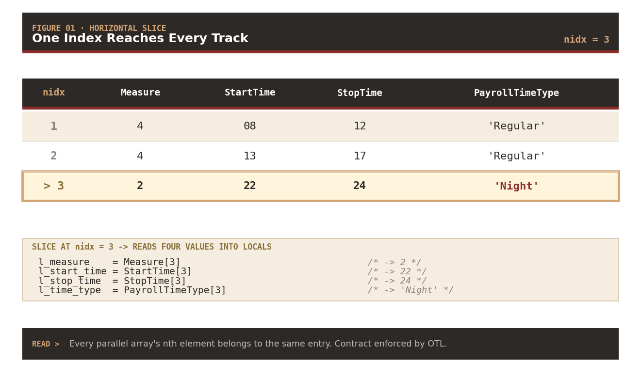
When OTL populates the DETAIL branch’s inputs, it doesn’t hand you one array of entry objects. It hands you a stack of parallel arrays, one array per attribute. Measure is one array. StartTime is another. PayrollTimeType is another. The contract that ties them together — the reason the pattern works at all — is that index k in every array refers to the same entry.
Think of it as a table lying on its side. Each parallel array is a column. Each entry is a row. When you set nidx = 3 and then read Measure[3], StartTime[3], and PayrollTimeType[3], you’re taking a horizontal slice — grabbing the third row’s cell from every column simultaneously. The three values you get back describe the same entry from three different angles.
Horizontal Slice at nidx = 3
| nidx | Measure | StartTime | StopTime | PayrollTimeType |
|---|---|---|---|---|
| 1 | 4 | 08 | 12 | 'Regular' |
| 2 | 4 | 13 | 17 | 'Regular' |
| ▸ 3 | 2 | 22 | 24 | 'Night' |
The slice at nidx=3 reads four values into locals:
l_measure    = Measure[3]           /* → 2 */
l_start_time = StartTime[3]         /* → 22 */
l_stop_time  = StopTime[3]          /* → 24 */
l_time_type  = PayrollTimeType[3]   /* → 'Night' */
One entry · four attributes · same index — All four locals now describe entry #3 from four angles: it’s a 2-hour night entry running 22:00 to 24:00. The alignment is guaranteed by OTL — it isn’t something the formula code has to verify. But the alignment only holds while nidx stays in-bounds.
The parallel-indexing contract is the reason no single “current entry” object exists. If you want everything about the entry, you take the horizontal slice yourself, reading every column at the same index. There’s no CurrentEntry.Measure — only Measure[nidx].
The Manual Increment — Why the Loop Body Owns It
Fast Formula’s WHILE has no auto-increment. There’s no FOR i IN 1..count equivalent. The loop condition is checked, the body runs, the condition is checked again — and if nothing inside the body changed the condition, you’re in an infinite loop. That’s why the increment line at the bottom of the body is mandatory:
nidx = 1

WHILE (nidx <= Measure.count) LOOP
(
  /* read the slice */
  l_measure = Measure[nidx]
  /* ... rest of body ... */

  nidx = nidx + 1   /* if you forget this, the loop never ends */
)
Two common mistakes deserve mentioning. First, the increment placed at the top of the body instead of the bottom — combined with an early return path — can skip the first entry. Second, the increment placed inside a conditional branch — IF condition THEN nidx = nidx + 1 — is exactly how an infinite loop reaches production. The increment always sits at the bottom of the body, always outside any conditional, always unconditional.
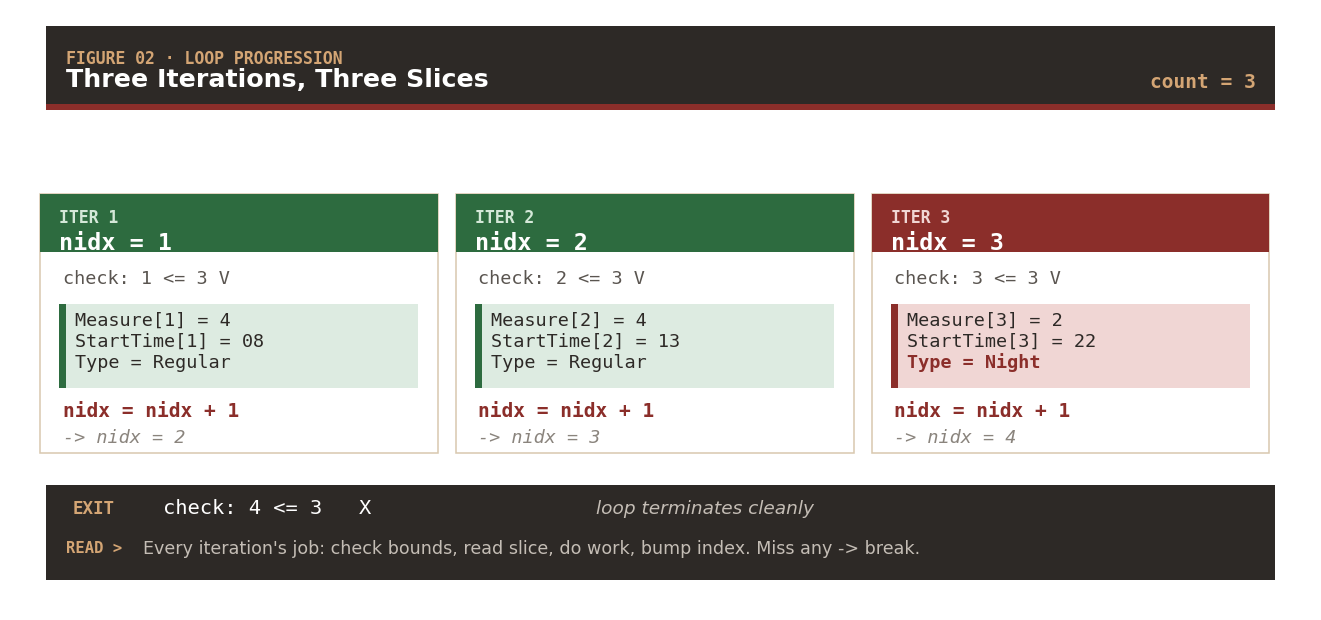
Three Iterations, Three Slices
For a three-entry day (Measure.count = 3), the loop runs three times and exits cleanly:
| Iteration | Enters when | Reads | Increments to |
|---|---|---|---|
| 1 | 1 <= 3 ✓ | Measure[1]=4, StartTime[1]=08, Type=Regular | nidx = 2 |
| 2 | 2 <= 3 ✓ | Measure[2]=4, StartTime[2]=13, Type=Regular | nidx = 3 |
| 3 | 3 <= 3 ✓ | Measure[3]=2, StartTime[3]=22, Type=Night | nidx = 4 |
| Exit | 4 <= 3 ✗ | — | loop terminates |
Termination depends on the increment — Remove the increment line and iteration 1 runs forever. The condition
nidx <= 3stays true because nothing ever changes nidx. That’s why the guard from Part 3 raises an error at nidx > 1000 — it’s a defense-in-depth against exactly this bug.
Every iteration’s job is the same: check bounds, read the slice, do the work, bump the index. The fourth step is what makes the loop finite. The parallel-array contract makes the second step efficient.
Bounds and the .exists() Safety Net
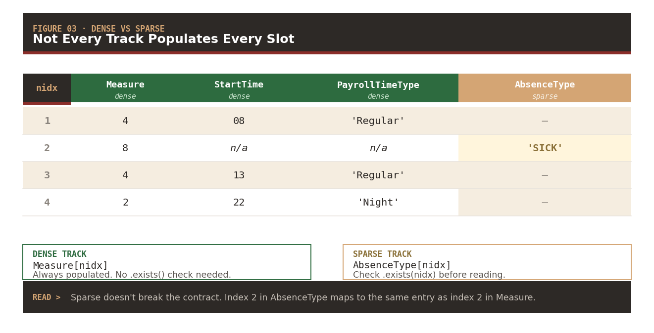
The obvious termination check is nidx <= Measure.count — perfect when every parallel array is dense (all indices from 1 to count are populated). Most of the primary tracks are dense: Measure, StartTime, StopTime, PayrollTimeType all populate for every entry. So looping until Measure.count is safe for the primary reads.
Where .exists() earns its keep is on the sparse arrays. Some tracks — AbsenceType is the canonical example — only carry a value at the indices where that attribute applies. For a day of five worked entries and one absence entry, AbsenceType has one populated element and five gaps. Reading AbsenceType[nidx] at a gap position throws — unless you check first:
IF (AbsenceType.exists(nidx)) THEN
(
  l_absence_type = AbsenceType[nidx]
  /* handle as absence entry */
)
ELSE
(
  /* handle as worked-time entry */
)
Dense vs Sparse — Same Contract, Different Populations
| nidx | Measure (dense) | StartTime (dense) | PayrollTimeType (dense) | AbsenceType (sparse) |
|---|---|---|---|---|
| 1 | 4 | 08 | 'Regular' | — |
| 2 | 8 | n/a | n/a | 'SICK' |
| 3 | 4 | 13 | 'Regular' | — |
| 4 | 2 | 22 | 'Night' | — |
- Dense track (
Measure[nidx]) — Always populated for every nidx from 1 to count. No.exists()check needed. - Sparse track (
AbsenceType[nidx]) — Populated only at entries that are absences. Always check.exists(nidx)before reading.
Sparse does not break the contract — Entry #2 above is an absence. Its dense tracks are filler; its sparse
AbsenceTypeis'SICK'. The parallel-indexing contract still holds — index 2 in AbsenceType maps to the same entry as index 2 in Measure. The sparse track just has gaps for entries where the attribute doesn’t apply.
Part 4 introduced AbsenceType as the sparse track. The reason .exists() exists is the sparse tracks. Every dense-only read can skip the guard; every sparse read needs it.
Complete Indexing Anatomy
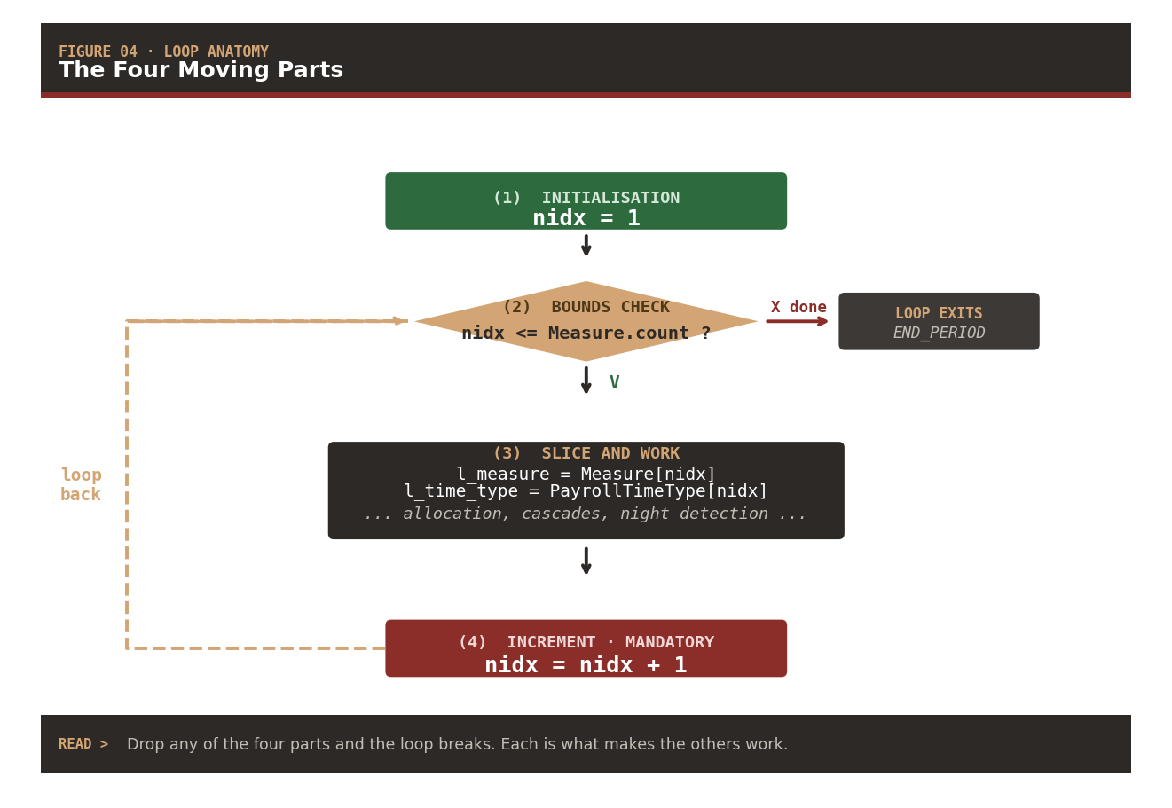
Pull it all together. The loop skeleton has four moving parts working in concert: initialization sets the index to 1, the bounds check decides whether to enter the body, the slice-and-work block reads the parallel arrays and does whatever the tier requires, and the increment at the bottom advances to the next entry.
① INITIALISATION
   nidx = 1
        │
        ▼
② BOUNDS CHECK ──── (fails) ───▶ LOOP EXITS
   nidx <= Measure.count?               (END_PERIOD)
        │
        │ (passes)
        ▼
③ SLICE AND WORK
   l_measure    = Measure[nidx]
   l_time_type  = PayrollTimeType[nidx]
   ... allocation, cascades, night detection ...
        │
        ▼
④ INCREMENT · MANDATORY
   nidx = nidx + 1
        │
        └──────── (loops back to ② ) ────────┘
Four parts · each one mandatory — Drop initialisation and nidx starts undefined. Drop the bounds check and the loop runs off the end of the array. Drop the slice-and-work body and nothing happens. Drop the increment and the loop never terminates. The pattern isn’t optional; each of the four parts is what makes the other three work.
This diagram is the shape of every DETAIL-phase iteration you write. The cascades, the night detection, the reconciliation, the trigger register — they all sit inside step ③. Steps ①, ②, and ④ are the skeleton that holds them.
Debug Pattern — Logging the Index
A single line at the top of every DETAIL iteration solves ninety percent of production debugging. Log nidx alongside the slice values you care about — l_measure, l_start_time, l_time_type. When something goes wrong for entry #7 of an eleven-entry day, having nidx in the log tells you exactly which slice to reason about:
ADD_RLOG(HWM_FFS_ID, HWM_RULE_ID,
         'ENTRY nidx=' || TO_CHAR(nidx) ||
         ' | measure=' || TO_CHAR(l_measure) ||
         ' | start='   || TO_CHAR(l_start_time) ||
         ' | type='    || l_time_type)
Every iteration produces one log line. The Analyze Rule Processing Details UI shows them in order, and searching for nidx=7 jumps straight to the entry in question. Cheap to add, effectively free at runtime, essential when a rule misbehaves for one entry out of many. Part 11 covers the ADD_RLOG mechanics — including the profile-level trap that makes these lines invisible if the log level isn’t set right.
Next in the Series · Series Finale
Part 11 — Debug Logging with ADD_RLOG, the Log Level Profile Trap, and the Final RETURN
The series closes with the two topics every TCR author eventually needs — how to log intermediate values so you can debug production issues, and how the final RETURN statement sends the outputs back to payroll.
Abhishek Mohanty · Oracle ACE Associate | AIOUG Member | Oracle HCM Cloud Consultant & Technical Lead — Fast Formulas, Absence Management, Time & Labor, Core HR, Redwood, HDL, OTBI.
TCR Deep Dive · Part 10 / 11 · Series tag: #TCRDeepDive